Turning it up is not the same as testing harder

A radiated immunity test is only as honest as its amplifier. The level setting is done once, with an unmodulated carrier, and every test level afterwards is worked out from it on the assumption that the amplifier behaves in a straight line. During the test the 80 % amplitude modulation pushes the peaks 1.8 times higher still. If the amplifier runs out of headroom anywhere along that chain, the field the product sees is not the field on the report, and nothing on the screen says so. The saturation check and the harmonics check are there to catch exactly that.

How the test level is set: calculated, not measured

The level setting of IEC 61000-4-3 is carried out with an unmodulated carrier at a field strength E_L of at least 1.8 times the test level E_T. A 10 V/m test is therefore level-set at 18 V/m, and the 80 % AM peaks of the test bring the field back up to that level. The test power is never set by watching the probe during the test: it is calculated from one sweep at constant power, in which the power that gives 18 V/m at a start point is recorded and the same power is then applied at the other fifteen points. The standard describes two ways of doing the level setting, the constant field strength method (clause 6.3.2) and the constant power method (clause 6.3.3). Everything shown here follows the constant power method. Step through it below, choose a test level, compare the calculated test field with the calibration field, and see on the amplifier gain plot how the test power is worked out from the power recorded at that frequency.

The saturation check: is the gain line straight?

Look again at the gain plot above. The test point P_T is found by sliding down the gain line by Δ dB from the recorded point P_c, and the generator is moved by the same Δ. That step is only right if the line is straight: the gain at P_T must be the gain measured at P_c. Nothing in the test checks this afterwards. Nobody puts a probe back in the field during the test; the power is simply applied.

The modulation then asks for more. With 80 % AM the peaks are 1.8 times the carrier, 5.1 dB higher, so during a 10 V/m test the amplifier is driven up to the power that gave 18 V/m in the level setting. If the gain line bends over anywhere in that stretch, the peaks come out short and the product sees less than the report says. The whole method stands or falls on one assumption: the amplifier gain stays constant over the range of power that is actually used. The saturation check is how IEC 61000-4-3 tests that assumption.

The check is simple and it is done at every level-setting frequency. P_L is the forward power that gives E_L = 18 V/m at the lowest field point, P_c + 20·log(18 / E_low) in the simulator's terms; it is the top of the range the test will use. With the signal generator at the level that produced P_L, reduce it by 5.1 dB, the same ratio as E_L/1.8, and record the new forward power. The step is not arbitrary: it covers exactly the stretch of the gain line between the modulation peaks of a 10 V/m test and its carrier. The difference between P_L and the new reading has to be between 3.1 dB and 7.1 dB. If it is, the amplifier is considered sufficiently linear and the system is suitable for testing. If it is not, the system is not suitable for testing at that frequency and level.

P1dB, the 1 dB compression point, is the output power at which the amplifier's gain has fallen 1 dB below its small-signal value. Below it the amplifier is close to linear: a change at the input gives the same change at the output. Above it every extra dB of drive gives less than a dB of output, until the amplifier saturates and gives almost nothing more. It is the figure amplifier data sheets quote for linear power. For 80 % AM the modulation peaks are 5.1 dB above the unmodulated carrier, so to keep the peaks at or below P1dB the carrier itself must sit about 5.1 dB below it. An amplifier whose P1dB rating only just covers the carrier power is already compressing the peaks it is meant to deliver.

• Less than 3.1 dB means the amplifier was already compressed at P_L: part of the level-setting power was never delivered in proportion, so the calculated test level and the modulation peaks cannot be trusted.
• More than 7.1 dB means the output fell further than the input, a non-linearity in the other direction, for example gain expansion or a level control acting in the amplifier.
• Edition matters. Edition 3.2 accepted 3.1 dB to 5.1 dB, and an interpretation sheet later accepted drops above 5.1 dB. Edition 4.0 writes the window as 3.1 dB to 7.1 dB, that is 5.1 dB ±2 dB.
• Other modulations need their own check. If anything other than 80 % AM is used, the standard asks for a saturation check based on the peak power of that modulated signal.

Edition 4.0 also adds Annex D.4, a fuller linearity check: the amplifier is stepped in 1 dB increments over the whole range actually used, including the 5.1 dB added for modulation, at least at the lowest, middle and highest frequency of each band, and its gain should stay within ±1 dB. It matters most when one level setting is used to derive several test levels, for example a 3 V/m test from a 10 V/m level setting, which spans the power needed for 1.67 V/m to 18 V/m. Move the test-level slider in the simulator down to 3 V/m and the gain plot shows why: the calculated point P_T is now far down the line, well away from the stretch that the 5.1 dB check looked at.

What saturation does to the test

The clearest way to see what saturation does is to look at the same 80 % AM signal twice: once through an amplifier with headroom to spare, and once through one that runs out of headroom at the modulation peaks. The top row is what the standard intends. The bottom row is what a product receives from a saturated amplifier.

Read across the rows and the difference is plain:

• Without saturation the spectrum holds exactly three lines: the carrier and one sideband 1 kHz either side, each −8 dB below the carrier. That is the signature of 80 % AM, and it is the only disturbance the product should see. There is nothing at 2f or 3f.
• In saturation the peaks are flattened, and the spectrum changes in two places at once. Around the carrier, new sidebands appear at ±2 kHz (−27 dB) and ±3 kHz (−40 dB): the harmonics of the 1 kHz modulation. And away from the carrier, lines appear at 2f (−37 dB) and 3f (−26 dB): the harmonics of the carrier itself, which the broadband field probe will add to its reading.
• The wanted sidebands shrink. The ±1 kHz sidebands fall to −9 dB, which means the modulation depth has dropped from 80 % to about 71 %. The energy that should have gone into modulating the product has gone into frequencies the standard never asked for.

For the test itself, that means:

• The peaks are cut off. The product receives a lower peak field than the report states, and a shallower modulation. For most products the demodulated 1 kHz signal is what causes the upset, so a shallower modulation is a gentler test.
• The level setting is wrong. If the amplifier is compressed during level setting, the forward-power data are built on an assumption of linearity that does not hold, and every test level calculated from them inherits the error.
• The disturbance is not the one defined. The extra 2 kHz and 3 kHz content, and the carrier harmonics, expose the product to signals the standard does not specify, which can cause failures or hide them.
• It can hide. Amplifiers with an output low-pass filter, or with internal combining that suppresses harmonics at the band edges, can be in saturation with no measurable carrier harmonics. The modulation sidebands at ±2 kHz and ±3 kHz are still there, which is why the 5.1 dB check is done on its own merits and not inferred from a clean spectrum. For such amplifiers Annex D suggests never exceeding the 2 dB compression point, at which the peak amplitude is already reduced by about 20 %.

The harmonics check: 6 dB below the fundamental

For every frequency at which the amplifier produces harmonics, they should be low enough that the harmonics in the electric field are at least 6 dB below the fundamental. Two details are easy to miss:

• It is the field that counts, not the amplifier output. The antenna is often far more efficient at the harmonic than at the fundamental, at the bottom of a band in particular. A typical broadband antenna has a noticeably higher gain and a much lower VSWR at 200 MHz than at 100 MHz: at 100 MHz a large part of the forward power is reflected back and what is accepted is radiated less effectively, while at 200 MHz almost all of it is accepted and radiated well. So when a 100 MHz test signal carries a second harmonic at 200 MHz, the antenna favours the harmonic, and a harmonic that looks acceptable at the amplifier output can be much stronger, relative to the fundamental, in the field. Annex D says as much: 6 dB at the amplifier may not be sufficient, depending on the antenna factor.
• Look at the lower third of each band. Harmonics matter most at the low end of each amplifier band: up to about a third of the amplifier's maximum frequency, the second and third harmonics still fall inside the band the amplifier and antenna are built to deliver.

What harmonics do to the field probe reading

The field probes used for level setting are broadband. They do not know which frequency they are looking at: they respond to everything in the field and apply the correction factor for the frequency they were told. Harmonics are therefore counted as if they were fundamental. How much they add depends on the probe's detector: a probe that responds to true RMS adds the fields as powers, while a diode probe driven beyond its square-law region responds partly to the peak, and then the harmonic can add almost in full, depending on its phase. That is why Annex D speaks of an error of 10 % or more.

• The product is under-tested. Annex D gives the example of a 10 V/m broadband reading made up of 9 V/m of fundamental and 4.5 V/m of harmonics. The level setting stops when the probe reads the target, so the fundamental, the frequency on the report, ends up 10 % or more below it.
• The probe's correction is for the wrong frequency. The correction factor applied is the one for the fundamental. The probe's sensitivity at 2f or 3f can differ by a dB or more, which adds a further error the simple sums below do not include.
• The uniformity data are wrong. Harmonics have their own field pattern in the chamber, so the sixteen readings of the uniform field area mix two different fields, and the forward-power data taken from them describe neither.
• False failures. A product that is robust at the test frequency may fail at its harmonic. The failure is recorded against the wrong frequency and can lead to a redesign that was never needed.
• Receivers are a special case. Even very weak harmonics can overload a sensitive receiver: testing a 900 MHz receiver at 300 MHz puts the third harmonic straight into its band. Here 6 dB is not enough. Non-harmonic spurious outputs of the signal generator can do the same.

Try it: slide the harmonic level

The slider sets how strong the harmonics are in the field, relative to the fundamental, and shows what a probe that adds them as powers reports. The example laboratory level-sets at 18 V/m for a 10 V/m test, as IEC 61000-4-3 does for 80 % AM. The assumptions behind the numbers are listed under the figure.

What to check in your records

What it adds up to: uncertainty, compliance and the choice of amplifier

Saturation and harmonics work in the same direction. A compressed amplifier delivers less than the calculated test power and clips the modulation peaks; harmonics make the probe read field that is not at the test frequency. Either way the product sees less than the report says. They are handled differently, though. Saturation is dealt with by a check the standard makes compulsory: an amplifier that passes the 5.1 dB step is treated as linear enough, and nothing is carried into the budget for it, which is exactly why the check has to be done, and done at every level-setting frequency. Harmonics have no such gate. The 6 dB guidance sets a limit but leaves the error in place, and the Annex J example budget has no term for it. Slide the harmonics to the −6 dBc of the Annex D guidance and the bias alone is close to 1 dB, a third of the total, larger than every term in the budget except the field probe itself.

That is more than a question of a larger uncertainty figure. A report that states 10 V/m while the product saw 9 V/m does not describe the test that was carried out. For an accredited laboratory, ISO/IEC 17025 asks for every significant contribution to the uncertainty to be evaluated and for the validity of the results to be monitored; an under-test that nobody measured is neither. And the product that passed may simply not comply.

Much of this is decided the day the amplifier is chosen. Take a quick look around the market and you can see many brands of amplifier only quote a single output power, without saying whether it is saturated power or power the amplifier delivers linearly. Many leave P1dB out altogether. Harmonics are often not specified at all, and where they are, the figure may be a typical value at reduced power, or only 13 dB to 15 dB below the fundamental at the amplifier output. So before a data sheet is taken at its word, it is worth asking:

• Which power is the headline? Saturated power, rated power and P1dB can be 2 dB or more apart. The test needs the carrier plus 5.1 dB for the modulation peaks, delivered linearly, and only P1dB, or better, measured linearity, says whether that is there.
• Minimum or typical, and where in the band? A typical value, or one measured at a single frequency, says little about the bottom of the band, which is where the antenna is least efficient and the most power is asked for.
• Harmonics at which power? A harmonic figure quoted at reduced power, or without a stated power, says nothing about the level you will actually run at. And 13 dB to 15 dB at the amplifier output leaves little margin once the antenna starts to favour the harmonic in the field.

The amplifier is usually the single heaviest investment in a radiated immunity system, and a number on a data sheet is just a number. What a laboratory is really buying is the assurance that the number can be trusted, and that it has been verified.

That is the ground on which we pick what we sell. Two Teseq amplifiers cover the IEC 61000-4-3 range. Both are designed around what saturation and harmonics do to a test: linear power is what the headline figure states, harmonics are guaranteed at the worst case rather than at a comfortable back-off, and the software that drives them carries out the checks:

80 MHz to 1 GHzTeseq CBA 80M1G E series Class A, one band, four models. The headline power is the linear power: 100 W, 225 W, 450 W and 975 W at P1dB, with the saturated figure quoted separately. Harmonics are specified at P1dB, the worst case, at −20 dBc minimum, and the brochure prints the gain error curve with the P1dB line drawn on it.

0.8 GHz to 6 GHzTeseq CBA 6G D series Class A, 30 W to 400 W at P1dB, with a built-in calibrated directional coupler for forward power. The 200 W model specifies harmonics at P1dB as well: −17 dBc from 0.8 GHz to 1 GHz and −19 dBc from 1 GHz to 6 GHz, both minima, not typical values.

Test softwareNexio BAT-EMC The radiated immunity module carries out the level setting, and with it the 5.1 dB saturation check at every level-setting frequency, with the result kept beside the forward-power data. The Annex D.4 linearity steps and the 16-point field uniformity run from the same module, on the same drivers, and go into the report automatically.

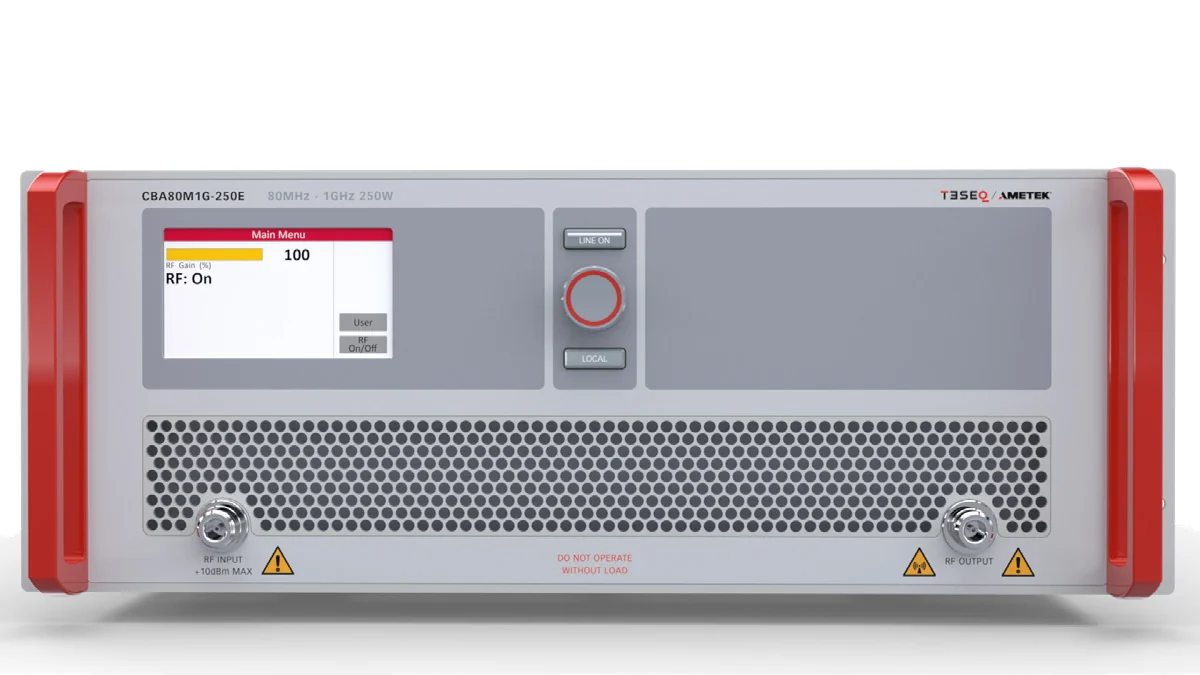
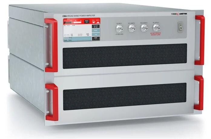
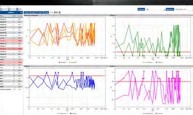
Both amplifiers are 100 % mismatch tolerant with no foldback, which matters at the bottom of the band where the antenna reflects most of what it is given, and both carry a three-year manufacturer's warranty. Figures are from the manufacturer's data sheets; the data sheet governs and specifications are subject to change.

The rest is our part of the work. We size the amplifier against your test plan rather than against a headline wattage, and the saturation check, the Annex D.4 linearity check and the harmonics can be run on your own system as part of a field uniformity verification, so the numbers are not just printed but shown, and are recorded every time the level setting is repeated rather than once at the time of purchase.